
The SUM function in excel is one of those features that have been around for ages. And if you have used Excel you are sure to use the function at least once. It is one of the most basic features in Excel and it functions to add values in Excel. As common as it is, this function is more prone to errors. Sometimes things just don’t add up and the SUM function doesn’t work.
In this guide, we will show you 6 reasons why this might happen and how you can troubleshoot the issues. But first, we will discuss some of the basic premises of the SUM function for you so that you understand how the SUM function works.
Basic Information on SUM
If you give some values to the SUM function it simply returns you with the summation of the values. SUM can take arrays, cell references, ranges, numbers, and constants. You can use these arguments in any combination. For example, you can add a range of numbers with cell references.
The SUM function will ignore text values in your series of numbers and will give you the sum of the numbers without any error. So, you can use SUM for cells containing texts without any worries.
Syntax
The syntax is very important to understand because it will help you understand why the SUM function is not working in some cases. In most cases, SUM does not work because you may not have followed the formula properly.
The syntax for the SUM function is
SUM(number1,[number2],…)
Syntax Breakdown
number1 represents the first number you wish to sum. This can be a number, a range such as A1:A50, or even a cell reference like A3.
number2 and onwards are optional arguments for the SUM function, and similar to number1, this can be a number, range, or a cell reference.
SUM Function Not Working: Reasons and Solutions
As we have said, often the primary reasons for SUM not working in Excel is a problem with the formula. But this is not always the case and SUM may not work due to default options in Excel.
We will show you some of the most common problems that you may encounter while working with SUM and provide solutions for them. So buckle up.
Selecting Cell References
Although we have said that SUM works with cell references. If you are putting in cell references as arguments for SUM, you may see that the SUM function is not working if you delete rows.
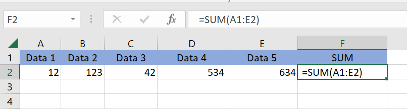
For example, we have a bunch of numbers in cells A2 through E2. And in the F2 cell, we have put the
SUM formula
=SUM(A2,B2,C2,D2,E2)
This will sum the individual values of each of the cell references as you can see in the picture.

But, if you have for some reason, deleted a row or a cell reference the SUM function will give you a #REF! error as you can see in the next image.

To fix this SUM function not working problem, use Cell ranges with SUM. This will give you an error-free calculation even if you delete any cell references or rows in a range. For SUM it is pretty simple, just enter the formula
=SUM()
In the parenthesis click, and use your mouse to drag and select the cells from A2 to E2 just like in the picture.

Now, if you have to delete a row, the SUM function will work and you won’t get an error. For our example, we have deleted the D row as shown in the picture.
As you can see the SUM function has automatically updated the cell ranges and now you’ve got a working SUM function.
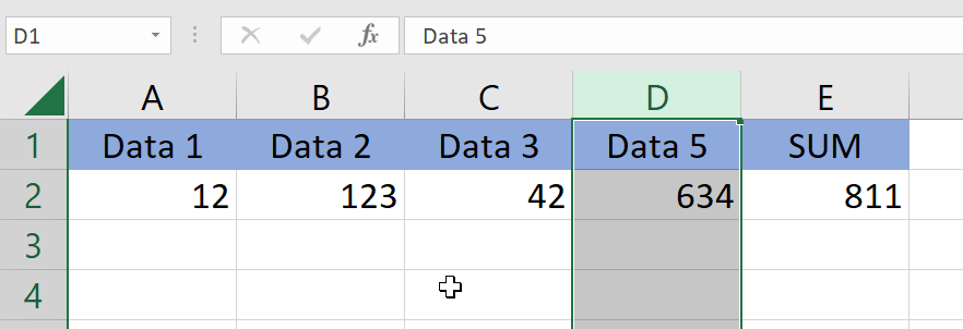
The most basic error that you may get is after writing the formula for SUM, the cell just outputs that formula. For example, in this case, we wanted to get the sum for cells ranging from A2 to E2.

As you can see the F2 cell where we wrote our formula shows the formula itself. It is a simple typo and happens because we didn’t put an equal sign before the formula. So Excel just shows the formula as is. To fix this SUM function not working error, just put in the equal sign and the function will work normally.

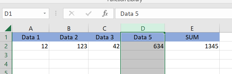
As you can see, with the equal sign the function works normally and shows the sum of the selected range.
SUM Not Working After You Deleted a Row
The SUM function may not work as you intended after you deleted a row from your workbook. For example, we have this sample data with 5 cells that we want to use SUM on. We write the correct SUM formula and we get the sum of the numbers.

But, for some reason, we may need to delete a row within the selected range. Say, we deleted the row D from this dataset.
Then we might find that the SUM function is not working and has not changed the sum to only 4 cells. Rather it kept the previous sum with the 5 cells.
This is a very common scene and can be fixed very easily. To fix this problem, just go to the Formulas tab on your Excel and on the far right hand corner click on Calculation Options. You may see that the Calculation Options is set to Manual and this is the culprit of this error.

Just click on Automatic to choose Automatic Calculation and then Excel will update the SUM value.
As you can see the SUM function is working correctly again after choosing the Automatic Calculation option.
You can also turn on Automatic Calculation from the Options menu in Excel. To do this, click on Files, and at the very bottom click on more and then options.

A new pop-up will appear. Click on the Formulas tab and ensure that the Automatic is checked.

And you are done. You should not get any more of those miscalculations in SUM.
A #NULL! Error
Another error you can get while working with SUM is a #NULL! Error. Often you will get this error due to a simple typing mistake. For this example, we wanted to get the sum of A2 through E2.

As you can see in this picture, in the formula bar we typed in
=SUM(A2 E2)
Although we wanted to select the range A2 to E2, we did not put in the semicolon. This resulted in the #NULL! Error. To fix this error, just put the semicolon in between the cell references like the image below and you’re set.

The SUM function will return the sum of the range without any errors.
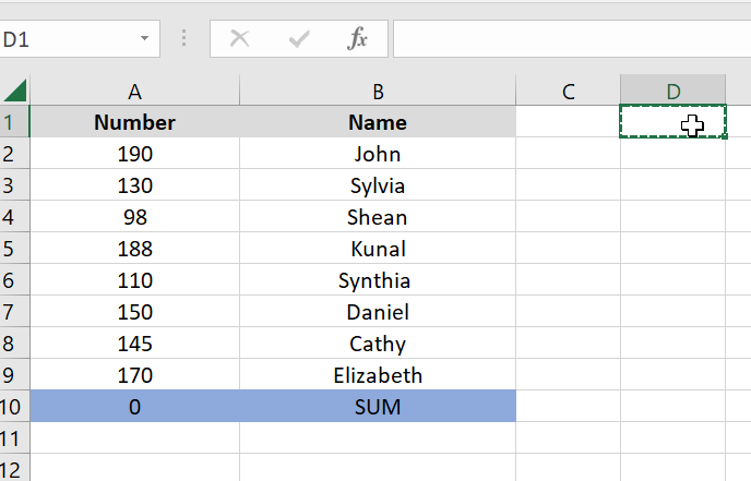
SUM Returning 0
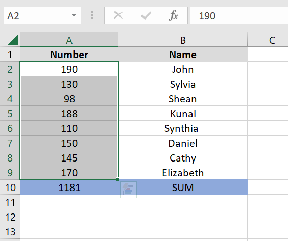
But what if you properly selected a range with a semicolon, and the formula is fine, but SUM is returning a 0. Well, this mostly happens when you are working with an imported dataset or you are editing someone else’s datasheet. If that’s the case, you may find that although you have written the formula correctly, SUM is still returning a 0.
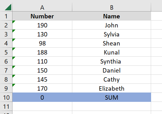
We have an example to show you how this can happen. For this example, we have names of some students and some numbers associated with them. We want to calculate the sum of the total numbers. And so, in the formula bar, we have typed the SUM formula:
=SUM(A2:A9)

This should have given us the sum of the numbers. But as you can see in the picture the SUM function returns a 0. This is a very common case if you are working with a document that you imported from somewhere. And most likely the culprit is that the value in the cells is stored as texts. To check this, click on any cell of the range.

As you can see from our image, there is an apostrophe sign before our number. In Excel, this means our number is stored as text. Don’t worry, this is easy to fix. You just have to simply convert the texts to numbers. To do this you can simply follow the various methods below.
Method 1: Using Text To Columns
To use this method, just follow the steps below:
1. First, select the range you want to change from text to numbers.
2. Click on your Data tab on Excel and select Text to Columns as marked on the picture below.

3. On the next menu that appears, click on Finish as shown in the image below

And you are done. All the text values in the selected range is converted into numbers. And you should get your sum instead of a 0
As you can see in the output, we have the sum of the numbers without any errors.
Method 2: Paste Special
For the second method you can just use the Paste special option in Excel. To do this, you can follow the process:
1. First, click on any empty cell and press CTRL+C to copy.
2. Then select the range you want to convert your texts to numbers by dragging with your mouse and click on the right mouse button as shown in the picture. Then, choose the Paste Special option.

3. On the next pop-up menu click on Values and Add as shown in the picture and press OK.

4. And you’re all set. And now, as you can see in the next image, the texts are converted into numbers and Excel has returned the SUM.

Method 3: Using Excel’s Smart Feature
As we have said in our guides time and time before, Excel is a very smart application. And often in situations like SUM function not working, Excel will smartly analyze the situation and give you a solution. For this example, we have the same dataset, but Excel is showing tiny green triangles in the corners of each number as you can see in the image.
These green triangles indicate that Excel recognizes that the numbers are stored as text. Similar to the previous situations SUM is returning a 0. To fix this using Excel’s smart suggestion feature, just follow along with this guide.
1. First, select the range of numbers with the green triangles. You will see that Excel shows you an icon in the right hand corner of your selection like the image below.

2. If you press on the icon a new pop up appears which will tell you that Excel recognizes that the cells contain numbers stored as texts and gives you a bunch of options.

3. The first suggestion that Excel gives you is to convert the texts to numbers. Click on that option and Bam! Excel will convert the texts to numbers.

As you can see, you now have converted the texts into numbers and SUM will show you the sum of the numbers.
Method 4: Using the VALUE Function
We can also use the value function to determine the value of the cells and then use SUM to add them together. To do this, just follow our guide.
1. First, click on an adjacent cell, and in the formula bar enter
=VALUE()
2. Inside the parenthesis, enter the first cell that is storing a text as a number. In our case, we selected A2 as the image below.

3. As you can see, the VALUE function returned the value of the cell. Now, hover with your mouse in the bottom left corner.
4. When you see the copy handler, simply click and drag the copy handler to the bottom of your cell range where the numbers are written up as text to copy the VALUE formula to these cells.

5. Now you will see that the texts have converted into numbers and you can get the SUM of the numbers. Now you can do a SUM function below this cell range with the SUM formula.

Cell Showing Formulas Only
Although this is a rare case and will only happen if you have accidentally changed this setting in Excel, you may see the SUM function you wrote in the formula bar exactly in the cell.
This can happen because of two cases.
Case 1
The first case where your cell is showing you the formula is because the Show Formulas option is turned on. To fix this, just follow these steps:
1. Click on the Formulas tab in your Excel.
2. Then on the far right see if the Show Formulas button is checked. If yes, just click on the button again and it will be unchecked.

3. This will solve your problem and you will get the SUM in your desired cell as you can see in the image here.

Case 2
The second case for your cell to show you only the formula is because you added an extra space before putting an equal sign in the formula bar. This is the case in our example image here.
Although this is very hard to catch, if you are careful you can avoid this and get the correct SUM value if you remove the spaces before the equal (=) sign.
Circular Reference Error
Although this is a super rare case, you may find yourself with a dialogue box that says
“There are one or more circular references where a formula refers to its own cell either directly or indirectly.”
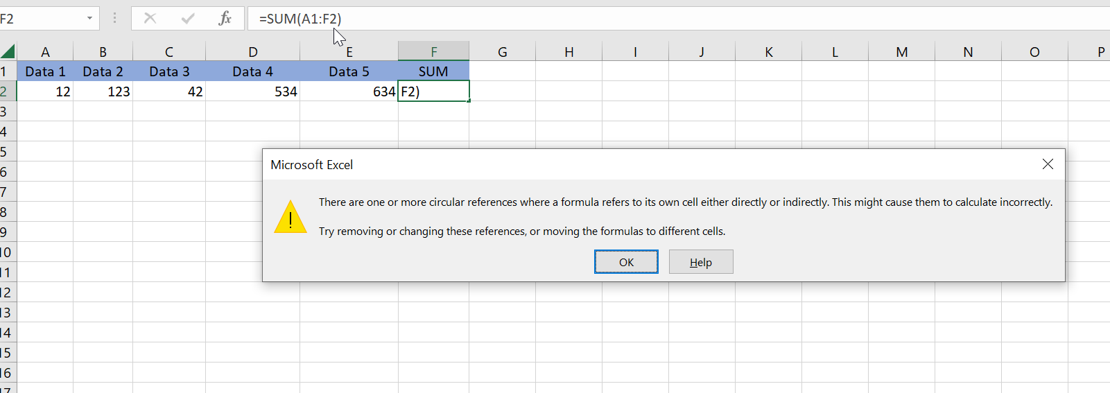
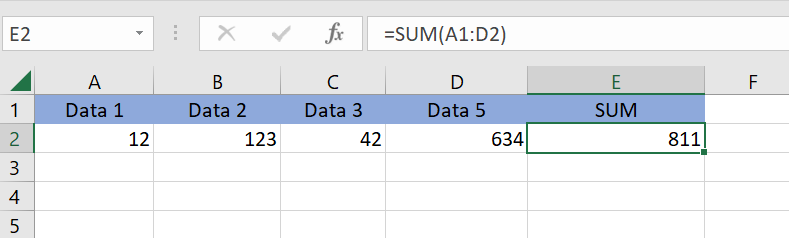
This happens mostly when you are trying to define a range for your SUM and you accidentally include the cell that contains the SUM formula. In our case, we were trying to get our SUM in the F2 cell and selected the F2 cell in the SUM argument.
To fix this, you just have to be careful not to enter the cell with the SUM formula in the SUM argument.
To Finish Up
In this guide we have provided you with some of the most common problems and errors that you may face where SUM function is not working in Excel. We have talked about some basic problems that may occur from silly typos. We also talked about some uncommon scenarios and errors that you may face while using the function.
Most of these errors can be fixed with some simple solutions as we have shown in our guide. But others need your careful practice of the solutions that we have shown here. If you follow this guide, then you should not face a problem with the Excel SUM function not working anymore.
If you have any further problems where your Excel SUM function is not working, just leave us a comment and we’ll be there to answer. Now have a blast and keep adding with SUM.
Similar Post: