
Combining multiple strings in Excel is a part of the job for any Excel user. The CONCATENATE function is there to help you with the process. But when you need to do the complete reverse and split a string of text into multiple strings, things get challenging. We will show you in this article the best methods to do the opposite of CONCATENATE in Excel.
Excel allows you to do a specific job in many ways. For instance, when splitting a string into many parts, you can manually write and input those strings. But it takes too long to do the job. Excel requires you to be more innovative and faster. We get this message and will discuss the four best methods you can use as reverse concatenation in Excel.
We will include visual demonstrations for all the methods. It will help you understand our explanations more effectively and faster than usual. After going through the guide, you will achieve the power to do the opposite of CONCATENATE in Excel in the shortest possible time.
Let’s get going!
What Does CONCATENATE Do in Excel?
It is essential to know what CONCATENATE is and what it does in Excel before discussing how we can do the opposite of it. Even if you know it, a short revision wouldn’t hurt. So let’s have a sneak peek into this function. Then we will dive into the opposite of CONCATENATE discussion.
The CONCATENATE function in Excel is self-explanatory; it conjoins multiple strings into a single string. Plus, it always returns strings in the text format. The function is mainly available in Excel 2021 and Excel for Microsoft 365 editions.
Let’s understand it with an example. See the image below. There are names in three parts: first, middle, and last. What to do if an Excel user needs to form Full Names from those separated names?

The CONCATENATE function is the best solution to join them and form the full name. Use this function to join all the names with spaces in between, and the result is foolproof!

See the output below.

One of the best things about this CONCATENATE function is that it lets you have nested formulas within itself. Therefore, the opportunity is there if you need to do concatenation with dynamic data strings.
I hope you have an idea of what the CONCATENATE does in Excel. But this article’s focus is on the opposite of CONCATENATE. So let’s move on and see reverse concatenation in upcoming sections.
What is the Opposite of CONCATENATE?
In the previous section, we showed what CONCATENATE means. There, we joined multiple strings into one string. So, it is straightforward to understand that the opposite of CONCATENATE in Excel refers to splitting a string into multiple strings.
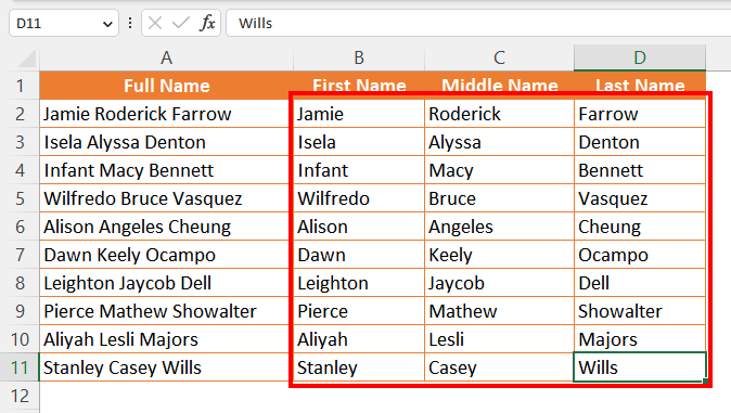
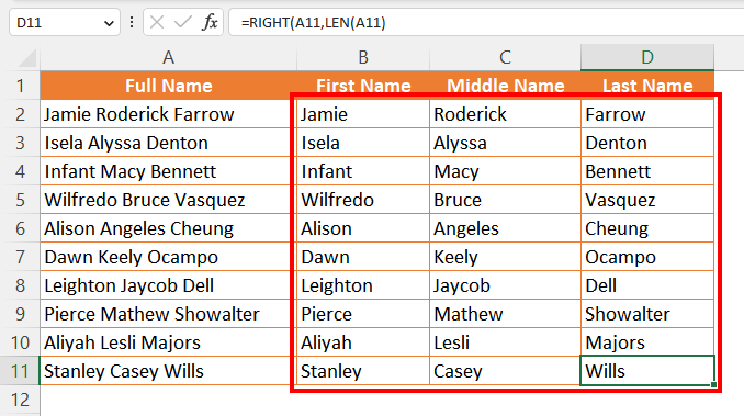
As always, let’s see an example here. The image below shows full names that need to be split into first, middle, and last names.
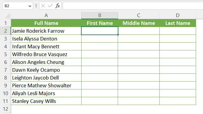
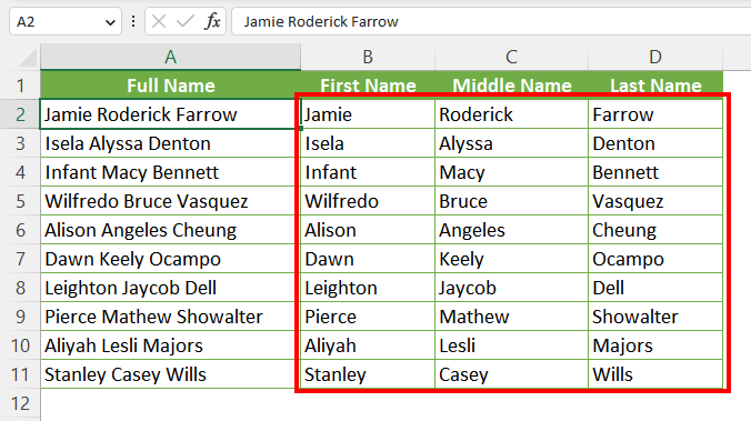
The opposite of concatenation will do precisely that. It would split a long string of text (full names here in this example) into multiple strings (first names, middle names, last names). The image below shows the final result.
But how to achieve the opposite of CONCATENATE in Excel? To know all about it, brace yourself and read the article’s next section carefully. In no time, you will learn more than one way to break a string of text into multiple parts!
4 Best Methods as the Opposite of CONCATENATE in Excel
You will always have several ways to do one task in Excel. That’s the beauty of this spreadsheet program. Irrespective of expertise level or difficulties, there is always a way for everyone to do a job in Excel.
It is no different in the Opposite of CONCATENATE discussion. We know quite a few ways to split a string into many parts. However, we decided to pick the four best methods to cover all Excel users. We also ensure that these methods are easy to follow and include visual demonstrations step-by-step.
Let’s begin with the first method!
Method 1: Using the Text to Columns Option
The Text to Columns option in Excel has been one of the best tools since its addition. A wizard menu takes you through the operation one step at a time. For the first method regarding the opposite of CONCATENATE in Excel, we could not help using this excellent option.
Now let’s see the process in steps.
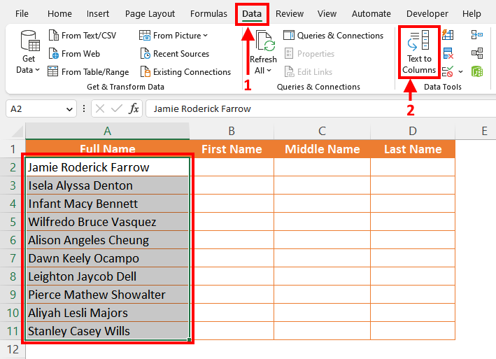
1. First, select your strings of text. Then go to the Data ribbon and find the Data Tools group. Then click on the Text to Columns button.
2. A Convert Text to Columns Wizard will open. Choose Delimited in the window and click the Next button.

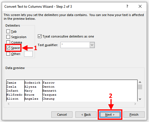
3. Select your delimiter in this window. Check the Space option if the parts in your text string are separated by space, like in this example (spaces separate the names). And if any other character, like a semicolon or comma, is used to separate parts of your string, select those in this list. Afterward, click the Next button.
4. You must select your destination columns for the split strings in this step. Click on the Destination box first. Then click and drag to select columns where you want your data, as marked (2) in the image below. As the final step here, click the Finish button.
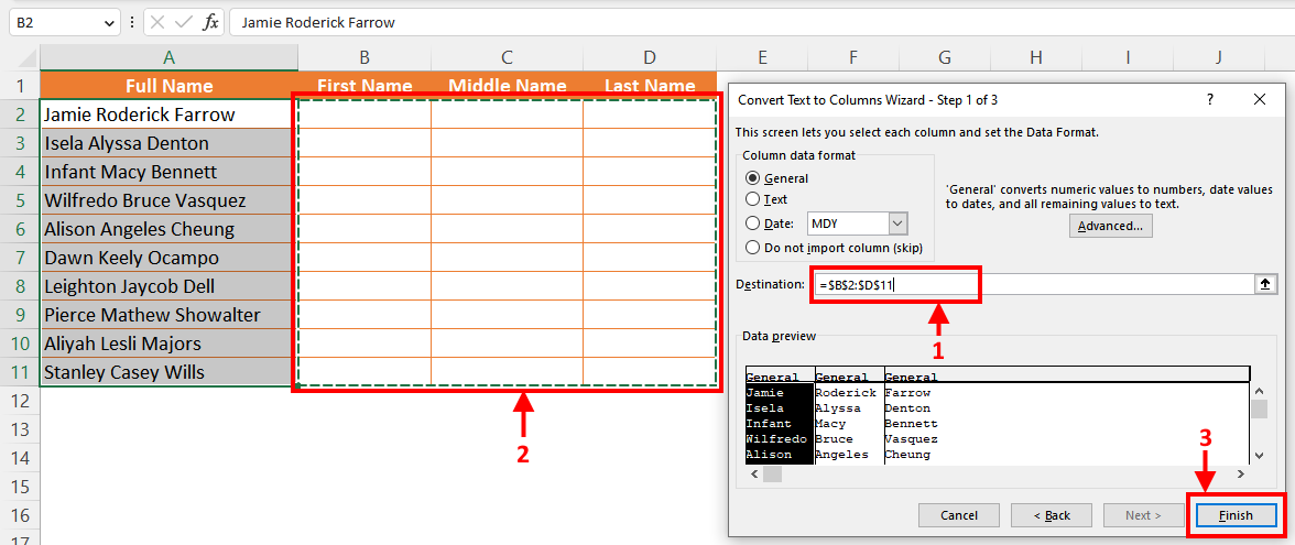
5. You will see a warning dialogue box. Click OK.

6. Eventually, you should see that your long strings of text have been cut into several parts following your selected delimiter(s) in the wizard window.
It is an excellent method for doing the opposite of CONCATENATE in Excel.
Method 2: Splitting Cell Values with Text Functions in Excel
Functions and formulas in Excel may seem daunting to many. But formulas make any job a whole lot easier and more effective. You are about to see another example of it in this method.
We will use the same dataset for this demonstration. Therefore, the objective is to split long strings of text (full names) into multiple strings (first, middle, and last names). We will use three sets of nested formulas to extract each part of the string. You can find all three formulas below.
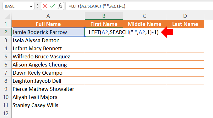
- First part of the string: =LEFT(A2,SEARCH(” “,A2,1)-1)
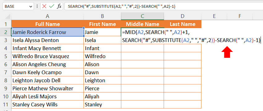
- Middle part of the string: =MID(A2,SEARCH(” “,A2)+1,SEARCH(“#”,SUBSTITUTE(A2,” “,”#”,2))-SEARCH(” “,A2)-1)
- Last part of the string: =RIGHT(A2,LEN(A2)-SEARCH(“#”,SUBSTITUTE(A2,” “,”#”,2)))
You can copy-paste the formulas for your use. You only need to change the Cell References in these formulas, A2. Change it to the cell name your string is in, and you will be fine!
Now let’s use these formulas and split a long string with three parts.
1. In this demonstration, the first part of the string is the first name. We wrote the formula =LEFT(A2,SEARCH(” “,A2,1)-1) and pressed the Enter button.
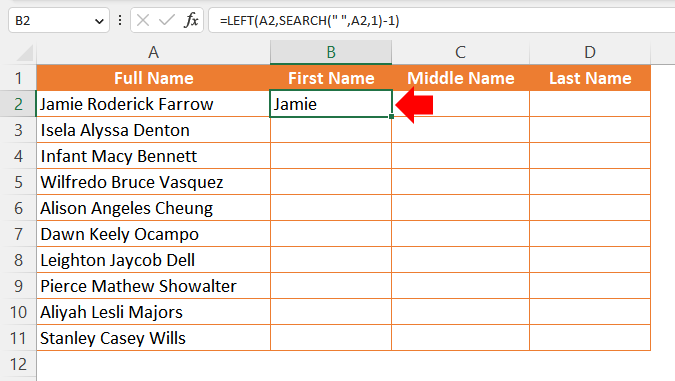
2. The formula extracted the first part of the name from cell A2, as it has been referenced here.
3. To split and extract the middle part of the string (middle name here), we wrote the formula =MID(A2,SEARCH(” “,A2)+1,SEARCH(“#”,SUBSTITUTE(A2,” “,”#”,2))-SEARCH(” “,A2)-1) and pressed the Enter key.
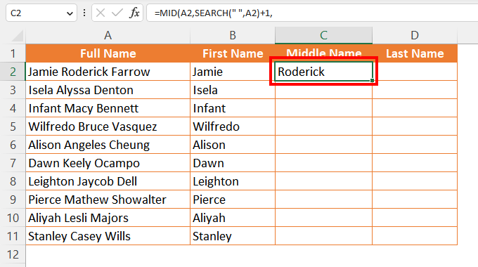
4. As a result, the formula has extracted the middle string.
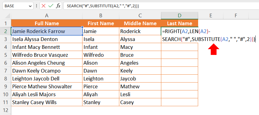
5. Now, for the third and final part of the string (last name here), we input the formula =RIGHT(A2,LEN(A2)-SEARCH(“#”,SUBSTITUTE(A2,” “,”#”,2))) and hit Enter.
6. Without any trouble, the formula extracted the last part of the string.
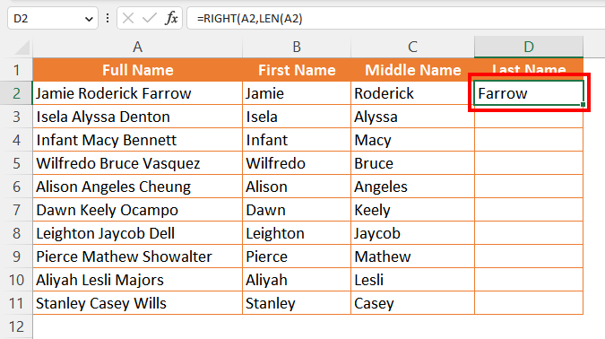
7. When all was done, we extracted multiple strings (first, middle, and last names) from a long string of text (full name).
It may seem troublesome initially if you are new to Excel and have little experience dealing with formulas. Don’t let it stop you. Practice the steps a few times, and you will get perfect results every time!
Method 3: With the TEXTSPLIT Function (Excel for Microsoft 365)
The TEXTSPLIT Function is Microsoft’s one of the latest additions to Excel. This function is exclusively available for Excel for Microsoft 365. However, the subscription fee is worth it for not only this function but for some other beautiful features and functions as well!
As a method for the opposite of CONCATENATE in Excel, the TEXTSPLIT function arrives at the scene with some magic up its sleeves. This function has dynamic array characteristics that make the whole splitting of text far more straightforward than it used to be. You need to select only your text (or cell reference it) and include your delimiter; the TEXTSPLIT will do the rest.
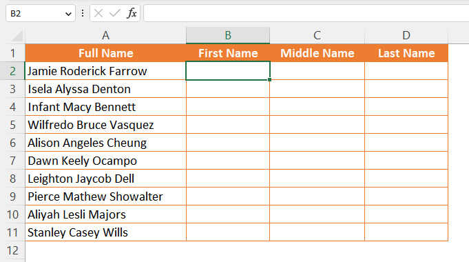
Let’s see the function in action with a fantastic demonstration. We are using the same dataset here too.
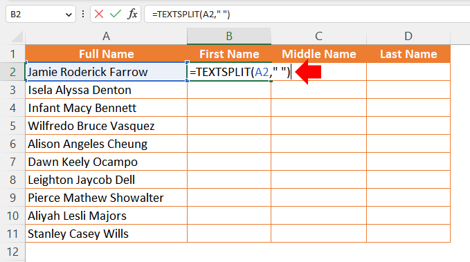
1. Select an empty cell and write the TEXTSPLIT formula. Here, we wrote =TEXTSPLIT(A2,“ ”). A2 is the cell reference, and “ ” is the space delimiter. When writing is done, press the Enter button.
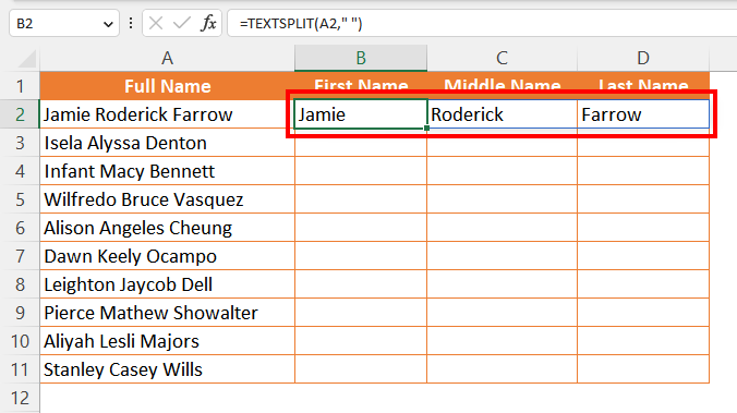
2. You should see that the whole text string has been separated by following the delimiter.
3. Fill up the column using the Fill Handle, and you are done!

Quick and easy!
Method 4: The Flash Fill Way
Flash Fill in Excel is a tool many are unaware of. Either they do not know how to use this option, or it is not enabled in their Excel program. The Flash Fill is also known as CTRL E. We have an article with some excellent use of this tool. Be sure to check it out.
We will use this super option as the opposite of CONCATENATE in Excel. It is fast and helpful in all cases. Even if you have a long string of text that you need to split into 10 or more parts, the Flash Fill allows you to do it in seconds!
The process is straightforward. Let’s see the demonstration below.
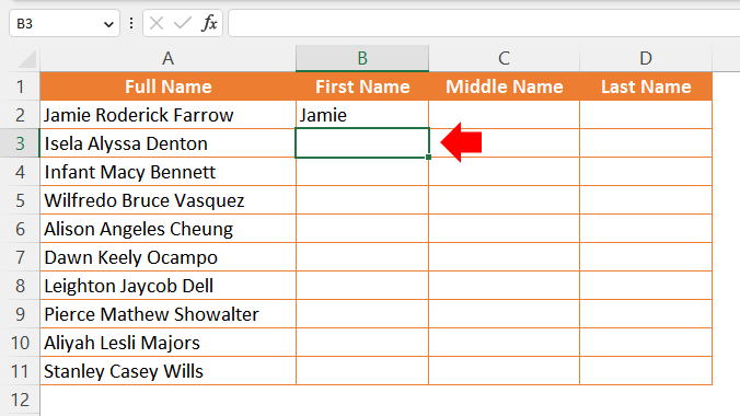
1. Select the first adjacent cell to your string of text. Then write the part you want to split from the long string. For instance, we will extract the first name here. After writing it, hit Enter.
2. The next cell down should be selected after pressing the Enter button. Do not do anything else. Press the CTRL+E buttons while the cell underneath your written string is still selected.
3. You will see that the first part of the string has been extracted from the long string!
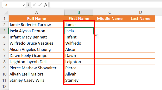
4. Follow the same process for the other parts of the strings.
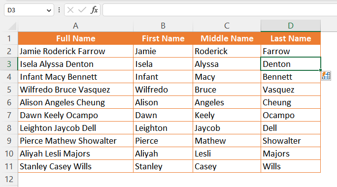
In the end, you will get a fully populated dataset with separated strings from your long text strings!
Important Tip: Always ensure that you are doing the Flash Fill in the adjacent columns. If there is any empty column in-between your source column with long strings and the destination column, the Flash Fill will not work.
Closing Thoughts
The Opposite of CONCATENATE in Excel is an excellent example concerning the necessity of knowing something inside-out in Excel. Most of the time, users face the dilemma of joining or merging multiple strings into one string. The topic of this article deals with how to do the opposite of it. Learning its methods will always help an Excel user in the long run.
We discussed four methods for reverse concatenating in Excel with visual demonstration. The first method may prove the most useful for all kinds of users. However, Method 2 and Method 3 are excellent choices for most professionals. And the last method, again, is for everyone to try and use.
As always, we strongly encourage you to practice all the methods a few times before deciding on your personal favorite. This way, you will know what works best for you and feel confident with your choice.
Keep on Excelling!
Similar Post: